Parallel Advantage
# Copyright 2026 Helge Gehring, Simon Bilodeau and contributors.
# Licensed under the Apache License, Version 2.0.
# ---
# jupyter:
#   jupytext:
#     text_representation:
#       extension: .py
#       format_name: percent
#       format_version: '1.3'
#   kernelspec:
#     display_name: Python 3
#     language: python
#     name: python3
# ---
Parallel Advantage
This example demonstrates the massive performance speedup achieved by leveraging
asynchronous cell generation in gdswell.
import time
from enum import Enum

import matplotlib.pyplot as plt
import numpy as np

import gdswell as gw


# Use a specific layer set
class Layers(gw.Layer, Enum):
    WG = (1, 0)
    LABEL = (10, 0)


@gw.cell
def complex_bend(radius: float, width: float = 2.0, n_points: int = 10000) -> gw.Cell:
    """
    A heavy cell that simulates complex geometry generation.
    """
    # Simulate heavy compute with a pure Python loop
    x = 0.0
    for i in range(10000_000):
        x += (i * 0.1) ** 0.5
    _ = x

    c = gw.Cell()

    # Generate a complex path (a spiral arc)
    t = np.linspace(0, np.pi / 2, n_points)
    src_pts = np.vstack([radius * np.cos(t), radius * np.sin(t)]).T

    # Simple "offset" to create a polygon representing a waveguide bend
    inner = src_pts * (1 - width / (2 * radius))
    outer = src_pts[::-1] * (1 + width / (2 * radius))

    poly_pts = [tuple(p) for p in np.concatenate([inner, outer])]
    c.add_polygon(poly_pts, layer=Layers.WG)

    return c
Benchmarking Performance
We will generate 40 complex bends first synchronously (one by one) and then asynchronously (in parallel).
# Number of heavy components to generate
count = 40
radii = [20.0 + i * 10.0 for i in range(count)]

print(f"--- GDswell Parallel Advantage Demo (Generating {count} heavy cells) ---")

# 1. Measurement: Synchronous (Blocking)
gw.config.async_cells = False
gw.clear_cache()

print("0. Baseline: Measuring a single synchronous build...")
start_baseline = time.perf_counter()
with gw.Layout() as _baseline_ly:
    _ = complex_bend(radii[0])
single_cell_time = time.perf_counter() - start_baseline
theoretical_sync_time = single_cell_time * count

print(f"   - Single cell sync build: {single_cell_time:.4f}s")
print(f"   - Estimated total sync time: {theoretical_sync_time:.2f}s")

# 2. Measurement: Asynchronous (Parallel)
gw.config.async_cells = True
gw.clear_cache()

print("\n1. Launching parallel build...")
start_async = time.perf_counter()
with gw.Layout() as layout:
    # Launch all tasks in background threads
    futures = [complex_bend(r) for r in radii]

    print(f"   - Launched {count} tasks in parallel.")

    # Assemble the layout
    top = gw.Cell()
    for i, f in enumerate(futures):
        top.add_ref(f, origin=(i * 20.0, i * 20.0))

    actual_async_time = time.perf_counter() - start_async
    print(f"   - Total parallel session time: {actual_async_time:.2f}s")
--- GDswell Parallel Advantage Demo (Generating 40 heavy cells) ---
0. Baseline: Measuring a single synchronous build...
   - Single cell sync build: 0.8860s
   - Estimated total sync time: 35.44s

1. Launching parallel build...
- Launched 40 tasks in parallel.
- Total parallel session time: 36.63s
Results Visualization
The chart below compares the theoretical synchronous execution time against the actual parallel execution time.
speedup = theoretical_sync_time / actual_async_time

# Plotting the results
labels = ["Synchronous (Estimated)", "Asynchronous (Actual)"]
times = [theoretical_sync_time, actual_async_time]

fig, ax = plt.subplots(figsize=(10, 6))
bars = ax.bar(labels, times, color=["#e74c3c", "#2ecc71"])

ax.set_ylabel("Time (seconds)")
ax.set_title(f"Performance Comparison: {count} Heavy Bends")
ax.grid(axis="y", linestyle="--", alpha=0.7)

# Add text labels on top of bars
for bar in bars:
    height = bar.get_height()
    ax.text(
        bar.get_x() + bar.get_width() / 2,
        height + 0.1,
        f"{height:.2f}s",
        ha="center",
        va="bottom",
        fontweight="bold",
    )

plt.figtext(
    0.5,
    0.01,
    f"Speedup: {speedup:.1f}x using parallel cell generation",
    ha="center",
    fontsize=12,
    bbox={"facecolor": "orange", "alpha": 0.2, "pad": 5},
)

plt.tight_layout()
plt.show()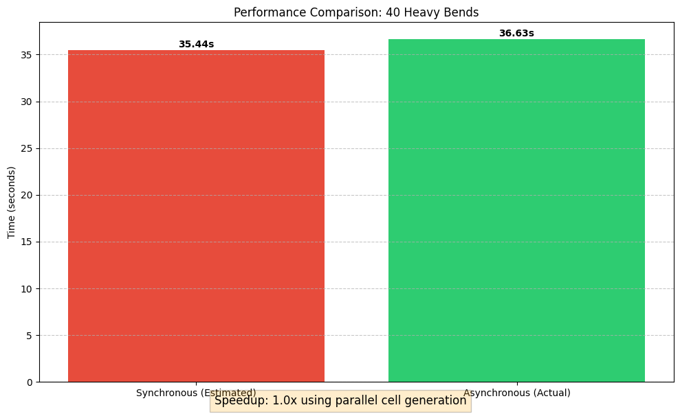
Layout Preview
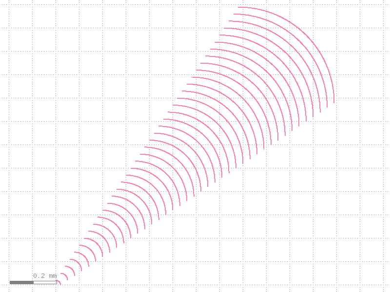
Here is the final generated layout with all parallel-generated components.
top