Time independent equation
\[
\left(
-\frac{\hbar^2}{2m} \frac{\mathrm{d^2}}{\mathrm{d}x^2} + V(x)
\right)
\varphi(x)
=
E
\varphi(x)
\]
Weak form with test function \(v\):
\[
\frac{\hbar^2}{2m}(\nabla \varphi, \nabla v)
+
V(x)(\varphi, v)
=
E (\varphi, v)
\]
Potential well
With
\[\begin{split}
V(x) =
\begin{cases}
0, &-L/2<&x&<L/2
\\
V_0 &\text{outside}
\end{cases}
\end{split}\]
we assemble a solution composed of
\[\begin{split}
\varphi(x) =
\begin{cases}
\varphi_1, &-L/2<&x
\\
\varphi_2, &-L/2<&x&<L/2
\\
\varphi_3, &&x&>L/2
\end{cases}
\end{split}\]
let
\[
k = \frac{\sqrt{2 m E}}{\hbar},
\quad
k^` = \frac{\sqrt{2 m (V_0 - E)}}{\hbar}
\text{and}
\quad
\alpha = \frac{\sqrt{2 m (V_0 - E)}}{\hbar}
\]
Inside the potential well
For inside the potential well this leads to
\[
\frac{\mathrm{d^2}}{\mathrm{d}x^2}
\varphi(x)
=
- k^2
\varphi(x)
\]
which can be solved using
\[
\varphi_2 = A \sin(k x) + B \cos(k x)
\]
Outside the potential well
and outside the potential well for unbound solutions, i.e. \(E>V_0\)
\[
\frac{\mathrm{d^2}}{\mathrm{d}x^2}
\varphi_{1/3}(x)
=
-{k^`}^2
\varphi_{1/3}(x)
\]
which can similary be solved using
\[
\varphi_{1/3} = C \sin(k^` x) + D \cos(k^` x)
\]
and bound solutions, i.e. \(E<V_0\)
\[
\frac{\mathrm{d^2}}{\mathrm{d}x^2}
\varphi_{1/3}(x)
=
\alpha^2
\varphi_{1/3}(x)
\]
solved by
\[
\varphi_1 = \mathrm{e}^{-F x} + \mathrm{e}^{G x}
\quad \text{and} \quad
\varphi_3 = \mathrm{e}^{-H x} + \mathrm{e}^{I x}
\]
Bound states
We find for the bound states,
i.e. states where we assume that \(\lim_{x\to\pm\inf}\varphi(x)=0\),
that the complete wavefunction simplifies to
\[\begin{split}
\varphi(x) =
\begin{cases}
\mathrm{e}^{G x}, &-L/2<&x
\\
A \sin(k x) + B \cos(k x), &-L/2<&x&<L/2
\\
\mathrm{e}^{-H x}, &&x&>L/2
\end{cases}
\end{split}\]
as the solutions need to be continous and differentiable, i.e.
\[
\varphi_1(-L/2) = \varphi_2(-L/2) \quad \varphi_2(L/2) = \varphi_3(L/2)
\]
and
\[
\left.\frac{\mathrm{d}\varphi_1}{\mathrm{d}x}\right|_{x=-L/2}
=
\left.\frac{\mathrm{d}\varphi_2}{\mathrm{d}x}\right|_{x=-L/2}
\quad
\text{and}
\quad
\left.\frac{\mathrm{d}\varphi_2}{\mathrm{d}x}\right|_{x=L/2}
=
\left.\frac{\mathrm{d}\varphi_3}{\mathrm{d}x}\right|_{x=L/2}
\]
which leads to \(A=0\) and \(G=H\) for the symmetric case and \(B=0\) and \(G=-H\) for the assymetric case.
this leads for the symmetric case to the conditions
\[\begin{split}
H \mathrm{e}^{-\alpha L/2} = B \cos(kL/2)
\text{ and }
-\alpha H \mathrm{e}^{-\alpha L/2} = - k B \sin(kL/2)
\\
\Rightarrow
\alpha = k \tan(kL/2)
\end{split}\]
and for the assymetric case to
\[\begin{split}
H \mathrm{e}^{-\alpha L/2} = B \sin(kL/2)
\text{ and }
-\alpha H \mathrm{e}^{-\alpha L/2} = k B \cos(kL/2)
\\
\Rightarrow
\alpha = - k \cot(kL/2)
\end{split}\]
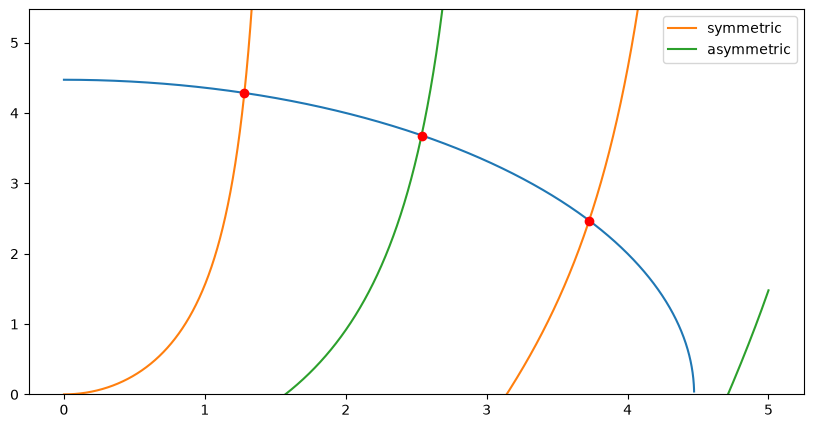
with \(u=\alpha L/2\) and \(v=kL/2\) and using \(u^2=u_0^2-v^2\) with \(u_0^2=mL^2V_0/2\hbar^2\) we can simplify both to
\[\begin{split}
\sqrt{u_0^2-v^2}
=
\begin{cases}
v \tan v, &\text{for the symmetric case}
\\
-v \cot v, &\text{for the asymmetric case}
\end{cases}
\end{split}\]