Bragg filter

Reproducing an example of [1] (and soon [2])

Show code cell source

Hide code cell source

from collections import OrderedDict

import matplotlib.pyplot as plt
import numpy as np
import shapely
from skfem import Basis, ElementTriP0
from skfem.io import from_meshio

from femwell.mesh import mesh_from_OrderedDict
from femwell.mode_solver_2d_periodic import plot_periodic, solve_periodic

height = 1
a = 0.330
b = 0.7
c = 0.2

k0 = 0.7 / a  # 1.05/a

left = shapely.LineString([(0, y) for y in np.linspace(-height, height, 20)])
right = shapely.LineString([(a, y) for y in np.linspace(-height, height, 20)])
top = shapely.LineString([(x, height) for x in np.linspace(0, a, 2)])
bottom = shapely.LineString([(x, -height) for x in np.linspace(0, a, 2)])

box = shapely.box(0, -height, a, height)
structure = shapely.box(0, -b / 2, a, b / 2)
hole = shapely.box(a / 4, -c / 2, a / 4 * 3, c / 2)

resolutions = {"hole": {"resolution": 0.1, "distance": 1}}

mesh = from_meshio(
    mesh_from_OrderedDict(
        OrderedDict(
            left=left,
            right=right,
            top=top,
            bottom=bottom,
            hole=hole,
            structure=structure,
            box=box,
        ),
        resolutions=resolutions,
        filename="mesh.msh",
        default_resolution_max=0.05,
        periodic_lines=[("left", "right")],
    )
)

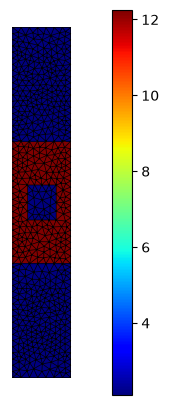
basis_epsilon_r = Basis(mesh, ElementTriP0(), intorder=4)

epsilon_r = basis_epsilon_r.zeros(dtype=np.complex64) + 1.45
epsilon_r[basis_epsilon_r.get_dofs(elements="structure")] = 3.5
epsilon_r **= 2
basis_epsilon_r.plot(np.real(epsilon_r), ax=mesh.draw(), colorbar=True).show()

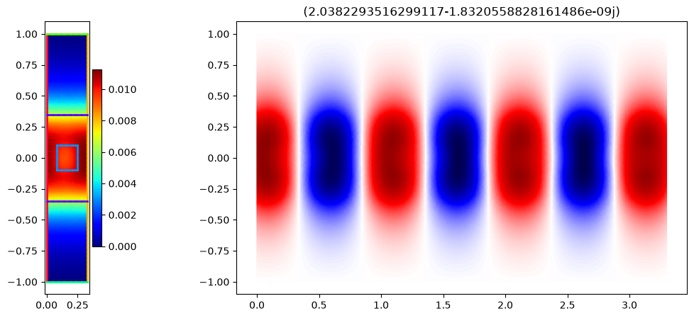
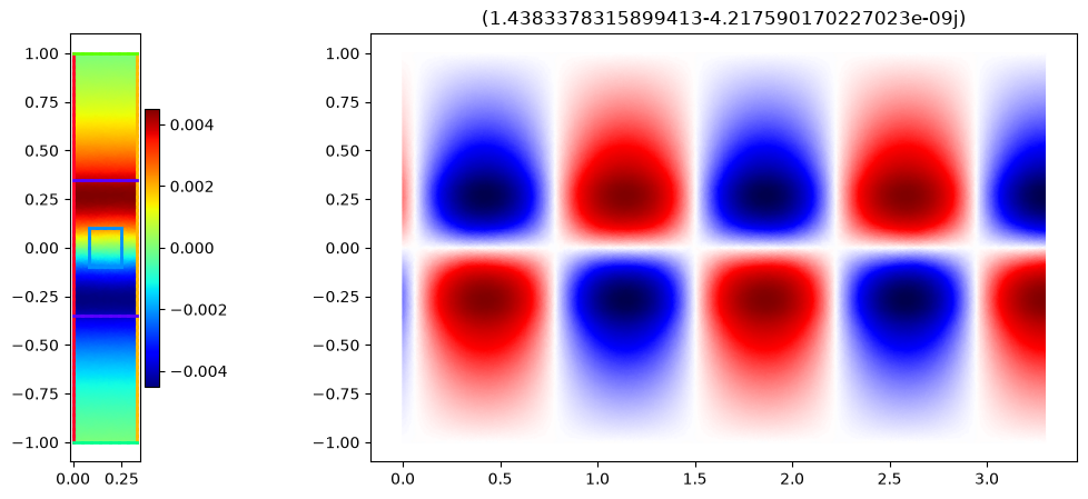
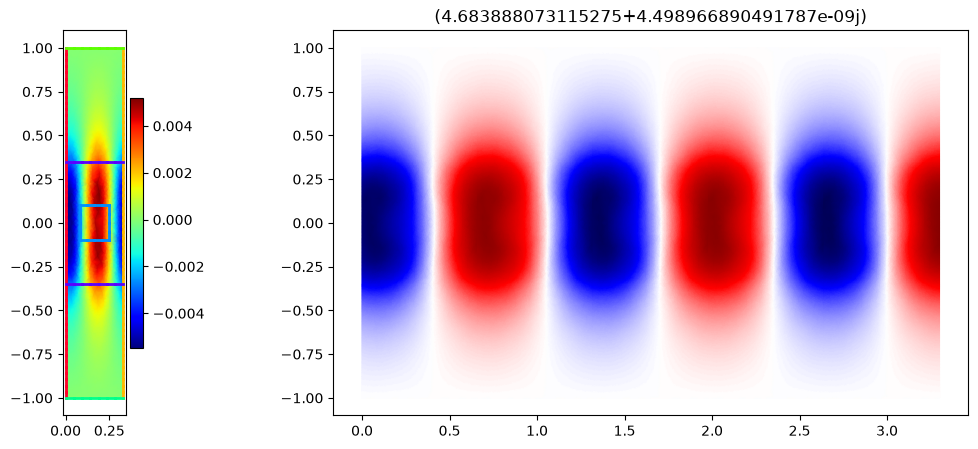
ks, basis_phi, phis = solve_periodic(basis_epsilon_r, epsilon_r, k0)


idx = np.abs(np.imag(ks * a)) < 0.5
ks = ks[idx]
phis = phis[:, idx]

# print(ks)

# plt.plot(np.real(ks))
# plt.plot(np.imag(ks))
# plt.show()

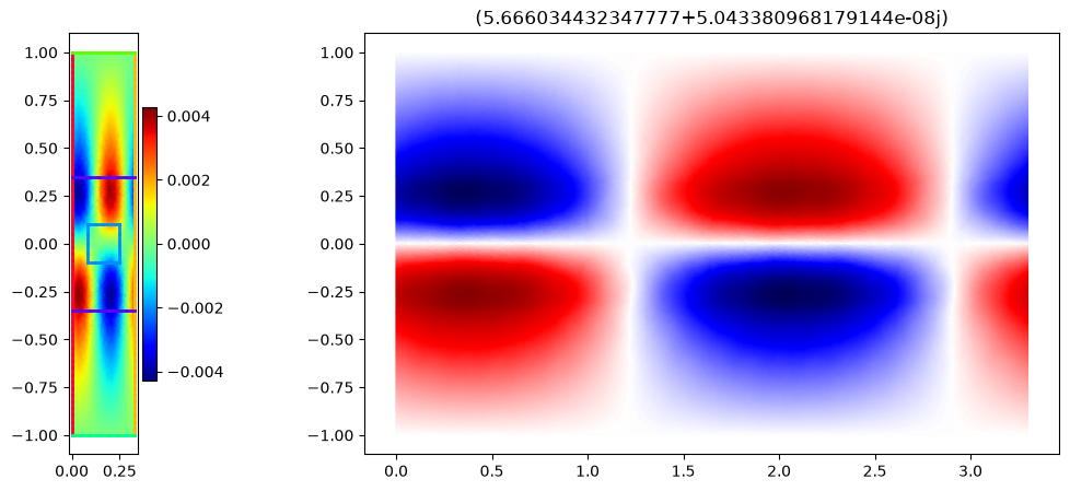
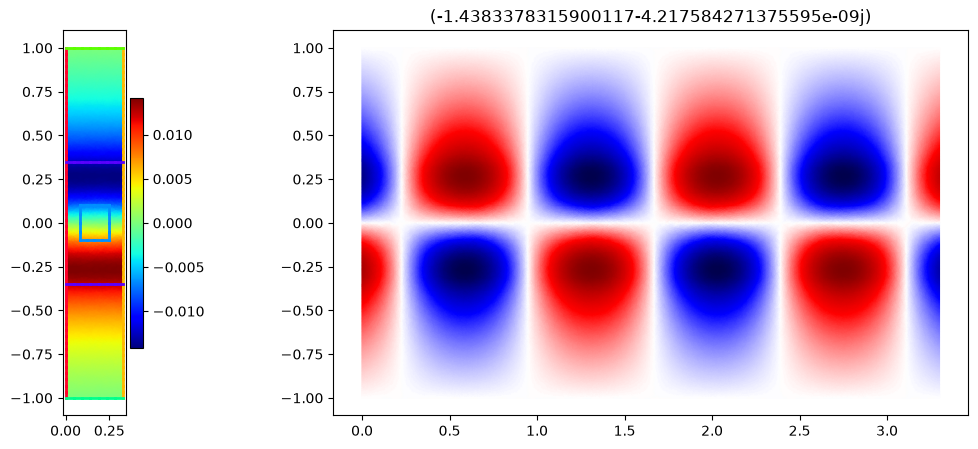
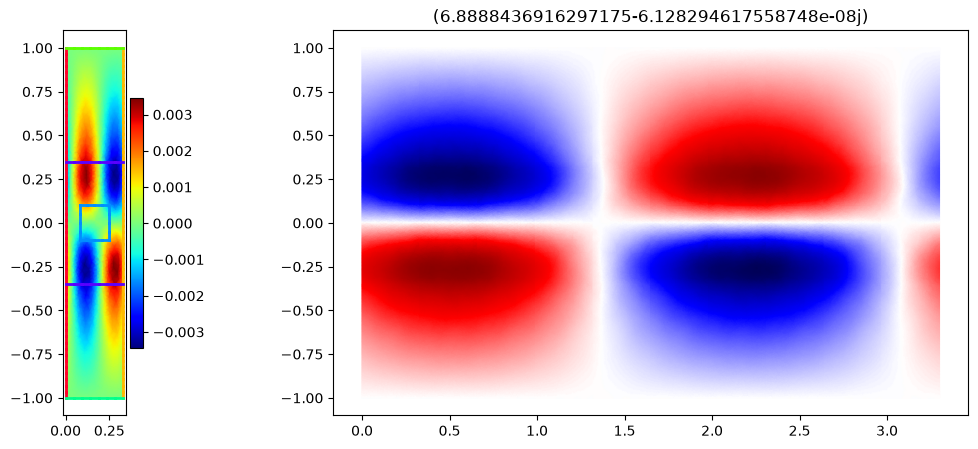
for i, k in enumerate(ks):
    fig, axs = plt.subplots(1, 2, figsize=(13, 5), gridspec_kw={"width_ratios": [1, 10]})
    mesh.draw(ax=axs[0], boundaries=True, boundaries_only=True)
    basis_phi.plot(np.real(phis[..., i]), shading="gouraud", colorbar=True, ax=axs[0])
    axs[0].set_aspect(1)
    plt.title(f"{k*a}")
    # axs[0].set_aspect(1)
    plot_periodic(k, a, basis_phi, phis[..., i], 10, axs[1])
    plt.show()

Bibliography

[1]

Jelena Notaros and Miloš A. Popović. Finite-difference complex-wavevector band structure solver for analysis and design of periodic radiative microphotonic structures. Optics Letters, 40(6):1053, March 2015. URL: https://doi.org/10.1364/ol.40.001053, doi:10.1364/ol.40.001053.

[2]

Chris Fietz, Yaroslav Urzhumov, and Gennady Shvets. Complex k band diagrams of 3d metamaterial/photonic crystals. Optics Express, 19(20):19027, September 2011. URL: http://dx.doi.org/10.1364/OE.19.019027, doi:10.1364/oe.19.019027.