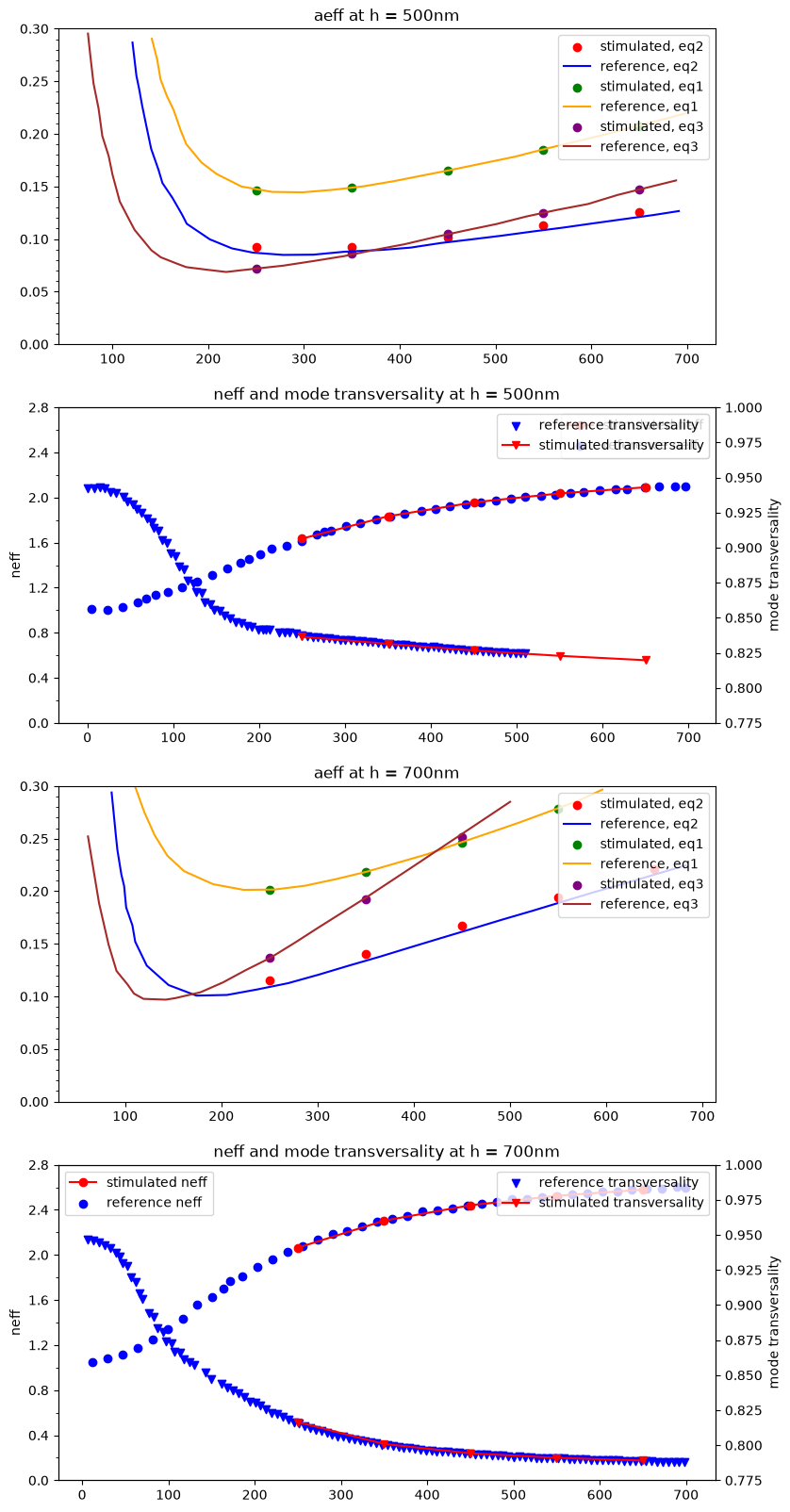
Effective area of a Si-NCs waveguide#
In this example we calculate the effective area and the effective refractive index of a Si-NCs waveguide from [1]
We describe the geometry using shapely. In this case it’s simple: we use a shapely.box for the waveguide according to the parameter provided in the paper For the surrounding we buffer the core and clip it to the part above the waveguide for the air Width is a sweep parameter from 50nm to 700nm
wavelength = 1.55
capital_w = 1.4
capital_h = 0.3
h_list = [0.5, 0.7]
t = 0.1
n_silicon = 3.48
n_air = 1
n_nc = 1.6
n_silica = 1.45
w_list = [x for x in range(250, 700, 100)]
neff_dict = dict()
aeff_dict = dict()
aeff1_dict = dict()
aeff3_dict = dict()
tm_dict = dict()
p_dict = dict()
for h in h_list:
    neff_list = []
    aeff_list = []
    aeff1_list = []
    aeff3_list = []
    tm_list = []
    p_list = []
    for width in w_list:
        width = width * 1e-3
        nc = shapely.geometry.box(
            -width / 2, capital_h + (h - t) / 2, +width / 2, capital_h + (h - t) / 2 + t
        )
        silica = shapely.geometry.box(-capital_w / 2, 0, +capital_w / 2, capital_h)
        silicon = shapely.geometry.box(-width / 2, capital_h, +width / 2, capital_h + h)

        polygons = OrderedDict(
            core=nc,
            silicon=silicon,
            silica=silica,
            air=nc.buffer(10.0, resolution=4),
        )

        resolutions = dict(
            core={"resolution": 0.02, "distance": 0.3},
            silicon={"resolution": 0.02, "distance": 0.1},
            silica={"resolution": 0.04, "distance": 0.5},
        )

        mesh = from_meshio(mesh_from_OrderedDict(polygons, resolutions, default_resolution_max=2))

        basis0 = Basis(mesh, ElementTriP0())
        epsilon = basis0.zeros()
        for subdomain, n in {
            "core": n_nc,
            "silicon": n_silicon,
            "air": n_air,
            "silica": n_silica,
        }.items():
            epsilon[basis0.get_dofs(elements=subdomain)] = n**2
        modes = compute_modes(basis0, epsilon, wavelength=wavelength, num_modes=3, order=1)

        for mode in modes:
            if mode.tm_fraction > 0.5:
                # mode.show("E", part="real")
                print(f"Effective refractive index: {mode.n_eff:.4f}")
                print(f"Effective mode area: {mode.calculate_effective_area(field='y'):.4f}")
                print(f"Mode transversality: {mode.transversality}")
                neff_list.append(np.real(mode.n_eff))
                aeff_list.append(mode.calculate_effective_area())
                tm_list.append(mode.transversality)
                p_list.append(mode.Sz)

                @Functional
                def I(w):
                    return 1

                @Functional
                def Sz(w):
                    return w["Sz"]

                @Functional
                def Sz2(w):
                    return w["Sz"] ** 2

                Sz_basis, Sz_vec = mode.Sz

                int_Sz = Sz.assemble(Sz_basis, Sz=Sz_basis.interpolate(Sz_vec))
                print("int(Sz)", int_Sz)  # 1 as it's normalized
                int_I = I.assemble(Sz_basis.with_elements("core"))
                print("int_core(1)", int_I)  # area of core

                int_Sz_core = Sz.assemble(
                    Sz_basis.with_elements("core"),
                    Sz=Sz_basis.with_elements("core").interpolate(Sz_vec),
                )
                print(
                    "int_core(Sz)",
                    int_Sz_core,
                )
                int_Sz2 = Sz2.assemble(Sz_basis, Sz=Sz_basis.interpolate(Sz_vec))
                print("int(Sz^2)", int_Sz2)

                aeff1_list.append(int_Sz**2 / int_Sz2)
                aeff3_list.append(int_I * int_Sz / int_Sz_core)
                break
        else:
            print(f"no TM mode found for {width}")
    neff_dict[str(h)] = neff_list
    aeff1_dict[str(h)] = aeff1_list
    aeff_dict[str(h)] = aeff_list
    aeff3_dict[str(h)] = aeff3_list
    tm_dict[str(h)] = tm_list
    p_dict[str(h)] = p_list
Plot the result
path = "../reference_data/Rukhlenko"

fig, axs = plt.subplots(4, 1, figsize=(9, 20))

for t1, t2, ax1, ax2 in [("0.5", "500", *axs[0:2]), ("0.7", "700", *axs[2:4])]:
    reference_neff = np.loadtxt(path + f"/fig_1c_neff/h_{t2}nm.csv", delimiter=",")
    reference_aeff1 = np.loadtxt(path + f"/fig_1b_aeff/{t1}_Eq1.csv", delimiter=",")
    reference_aeff2 = np.loadtxt(path + f"/fig_1b_aeff/{t1}_Eq2.csv", delimiter=",")
    reference_aeff3 = np.loadtxt(path + f"/fig_1b_aeff/{t1}_Eq3.csv", delimiter=",")
    reference_tm = np.loadtxt(path + f"/fig_1c_neff/tm_h_{t2}nm.csv", delimiter=",")

    ax1.scatter(w_list, aeff_dict[t1], c="r", label="stimulated, eq2")
    ax1.plot(reference_aeff2[:, 0], reference_aeff2[:, 1], c="b", label="reference, eq2")

    ax1.scatter(w_list, aeff1_dict[t1], c="green", label="stimulated, eq1")
    ax1.plot(reference_aeff1[:, 0], reference_aeff1[:, 1], c="orange", label="reference, eq1")

    ax1.scatter(w_list, aeff3_dict[t1], c="purple", label="stimulated, eq3")
    ax1.plot(reference_aeff3[:, 0], reference_aeff3[:, 1], c="brown", label="reference, eq3")

    ax1.set_title(f"aeff at h = {t2}nm")
    ax1.yaxis.set_major_locator(MultipleLocator(0.05))
    ax1.yaxis.set_minor_locator(MultipleLocator(0.01))
    ax1.set_ylim(0, 0.3)
    ax1.legend(loc="upper right")

    ax2b = ax2.twinx()
    ax2b.set_ylabel("mode transversality")
    ax2b.scatter(
        reference_tm[:, 0],
        reference_tm[:, 1],
        marker="v",
        c="b",
        label="reference transversality",
    )
    ax2b.plot(w_list, tm_dict[t1], "-v", c="r", label="stimulated transversality")
    ax2b.set_ylim(0.775, 1)
    ax2b.legend()

    ax2.plot(w_list, neff_dict[t1], "-o", c="r", label="stimulated neff")
    ax2.scatter(reference_neff[:, 0], reference_neff[:, 1], c="b", label="reference neff")
    ax2.set_title(f"neff and mode transversality at h = {t2}nm")
    ax2.set_ylabel("neff")
    ax2.yaxis.set_major_locator(MultipleLocator(0.4))
    ax2.yaxis.set_minor_locator(MultipleLocator(0.2))
    ax2.set_ylim(0, 2.8)
    ax2.legend()

plt.show()
/home/runner/miniconda3/lib/python3.13/site-packages/matplotlib/cbook.py:1810: ComplexWarning: Casting complex values to real discards the imaginary part
  return math.isfinite(val)
/home/runner/miniconda3/lib/python3.13/site-packages/matplotlib/collections.py:205: ComplexWarning: Casting complex values to real discards the imaginary part
  offsets = np.asanyarray(offsets, float)
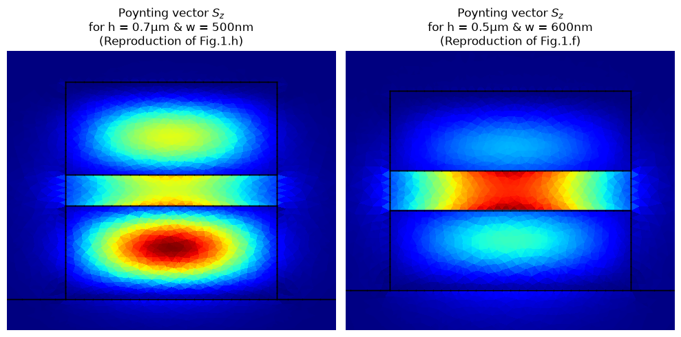
We can also plot the modes to compare them with the reference article
# Data figure h
w_fig_h = 500
idx_fig_h = min(range(len(w_list)), key=lambda x: abs(w_list[x] - w_fig_h))
h_fig_h = 0.7
basis_fig_h, Pz_fig_h = p_dict[str(h_fig_h)][idx_fig_h]

# Data figure f
w_fig_f = 600
idx_fig_f = min(range(len(w_list)), key=lambda x: abs(w_list[x] - w_fig_f))
h_fig_f = 0.5
basis_fig_f, Pz_fig_f = p_dict[str(h_fig_f)][idx_fig_f]

fig, ax = plt.subplots(1, 2)

basis_fig_h.plot(np.abs(Pz_fig_h), ax=ax[0], aspect="equal")
ax[0].set_title(
    f"Poynting vector $S_z$\nfor h = {h_fig_h}μm & w = {w_fig_h}nm\n(Reproduction of Fig.1.h)"
)
ax[0].set_xlim(-w_fig_h * 1e-3 / 2 - 0.1, w_fig_h * 1e-3 / 2 + 0.1)
ax[0].set_ylim(capital_h - 0.1, capital_h + h_fig_h + 0.1)
# Turn off the axis wrt to the article figure
ax[0].axis("off")
# Add the contour
for subdomain in basis_fig_h.mesh.subdomains.keys() - {"gmsh:bounding_entities"}:
    basis_fig_h.mesh.restrict(subdomain).draw(
        ax=ax[0], boundaries_only=True, color="k", linewidth=1.0
    )

basis_fig_f.plot(np.abs(Pz_fig_f), ax=ax[1], aspect="equal")
ax[1].set_title(
    f"Poynting vector $S_z$\nfor h = {h_fig_f}μm & w = {w_fig_f}nm\n(Reproduction of Fig.1.f)"
)
ax[1].set_xlim(-w_list[idx_fig_f] * 1e-3 / 2 - 0.1, w_list[idx_fig_f] * 1e-3 / 2 + 0.1)
ax[1].set_ylim(capital_h - 0.1, capital_h + h_fig_f + 0.1)
# Turn off the axis wrt to the article figure
ax[1].axis("off")
# Add the contour
for subdomain in basis_fig_f.mesh.subdomains.keys() - {"gmsh:bounding_entities"}:
    basis_fig_f.mesh.restrict(subdomain).draw(
        ax=ax[1], boundaries_only=True, color="k", linewidth=1.0
    )

fig.tight_layout()
plt.show()
Bibliography#
[1]
Ivan D. Rukhlenko, Malin Premaratne, and Govind P. Agrawal. Effective mode area and its optimization in silicon-nanocrystal waveguides. Optics Letters, 37(12):2295, June 2012. URL: http://dx.doi.org/10.1364/OL.37.002295, doi:10.1364/ol.37.002295.