Overlap with the mode of an optical fiber

Show code cell source

Hide code cell source

from collections import OrderedDict

import matplotlib.pyplot as plt
import numpy as np
from shapely import box
from skfem import Basis, ElementTriP0, ElementTriP1
from skfem.io import from_meshio
from tqdm import tqdm

from femwell.fiber import e_field_gaussian, overlap
from femwell.maxwell.waveguide import compute_modes
from femwell.mesh import mesh_from_OrderedDict

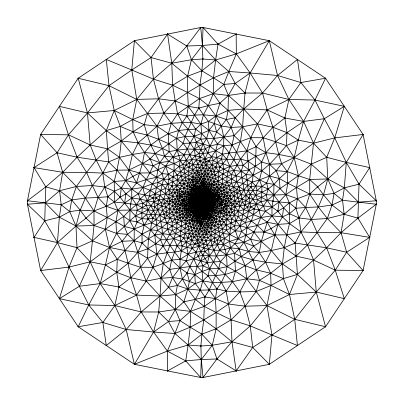
In this case the geometry is super simple: We just define a small waveguide surrounded by silicon oxide. As we later want to calculate overlap integrals, we put the waveguide centered at 0,0. We don’t need to simulate the whole fiber, just the are in which the field is non-zero.

core = box(-0.1, -0.15, 0.1, 0.15)
polygons = OrderedDict(core=core, clad=core.buffer(15, resolution=4))

resolutions = dict(core={"resolution": 0.01, "distance": 0.1})
mesh = from_meshio(mesh_from_OrderedDict(polygons, resolutions, default_resolution_max=10))
mesh.draw().show()

We choose as the core-material silicon nitride and for the cladding silicon dioxide. Accordingly, we set the refractive indices.

basis0 = Basis(mesh, ElementTriP0(), intorder=4)
epsilon = basis0.zeros().astype(complex)
epsilon[basis0.get_dofs(elements="core")] = 1.9963**2
epsilon[basis0.get_dofs(elements="clad")] = 1.444**2
# basis0.plot(np.real(epsilon), colorbar=True).show()

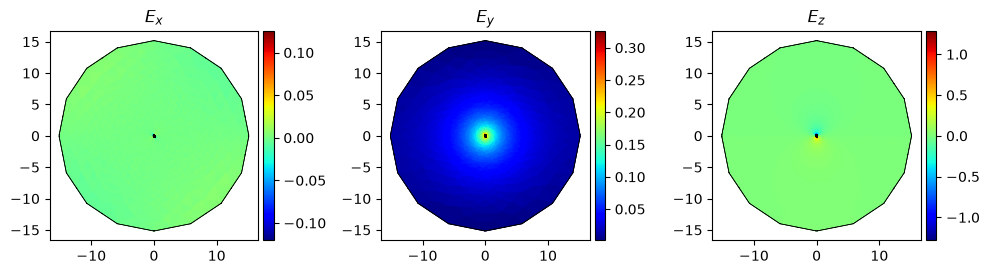
Now we simulate the mode of the small waveguide! We don’t use metallic boundary conditions, i.e. here a derivative of zero is enforced at the outer boundary of the simulation. Thus, we know, that we chose the cladding thick enough if the field vanishes at the outer boundaries.

modes = compute_modes(basis0, epsilon, wavelength=1.55, mu_r=1, num_modes=1)

fig, axs = modes[0].plot(modes[0].E.real, direction="x")
plt.tight_layout()
plt.show()

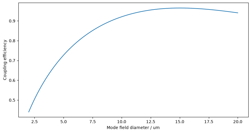
Now we sweep the mode-field-diameter of the fiber to see the dependence of the coupling on the MFD. As the waveguide is asymmetric, we get non-hybridized modes, i.e. either TE- or TM-modes. Thus, it’s sufficient to calculate the overlap with the non-zero in-plane component.

mfds = np.linspace(2, 20, 100)
efficiencies = []

for mfd in tqdm(mfds):
    basis_fiber = basis0.with_element(ElementTriP1())
    x_fiber = basis_fiber.project(
        lambda x: e_field_gaussian(np.sqrt(x[0] ** 2 + x[1] ** 2), 0, mfd / 2, 1, 1.55),
        dtype=complex,
    )

    efficiency = overlap(
        basis_fiber, modes[0].basis.interpolate(modes[0].E)[0][1], basis_fiber.interpolate(x_fiber)
    )
    efficiencies.append(efficiency)

plt.plot(mfds, efficiencies)
plt.xlabel("Mode field diameter / um")
plt.ylabel("Coupling efficiency")
plt.show()