Variation of the width

To understand the propagation in a waveguide, it’s often helpful to look at how the effective refractive indices of the modes change when adjusting the width of the waveguide. As the modes continously change their refractive index, we can track them through their evolution. We gray the area which would indicate a effective refractive index below the refractive index of the underlying layer (commonly refered to as box), as such modes would not be guided. The refractive index of the box called “cutoff”, as it defines the effective refractive index level under which modes stop being guided.

Show code cell source Hide code cell source

from collections import OrderedDict

import matplotlib.pyplot as plt
import numpy as np
from shapely.geometry import box
from shapely.ops import clip_by_rect
from skfem import Basis, ElementTriP0
from skfem.io.meshio import from_meshio
from tqdm import tqdm

from femwell.maxwell.waveguide import compute_modes
from femwell.mesh import mesh_from_OrderedDict

wavelength = 1.55
num_modes = 8
widths = np.linspace(0.5, 3.5, 100)

all_neffs = np.zeros((widths.shape[0], num_modes))
all_te_fracs = np.zeros((widths.shape[0], num_modes))
for i, width in enumerate(tqdm(widths)):
    core = box(0, 0, width, 0.33)
    polygons = OrderedDict(
        core=core,
        box=clip_by_rect(core.buffer(1.0, resolution=4), -np.inf, -np.inf, np.inf, 0),
        clad=clip_by_rect(core.buffer(1.0, resolution=4), -np.inf, 0, np.inf, np.inf),
    )

    resolutions = {"core": {"resolution": 0.1, "distance": 1}}

    mesh = from_meshio(mesh_from_OrderedDict(polygons, resolutions, default_resolution_max=0.6))

    basis0 = Basis(mesh, ElementTriP0())
    epsilon = basis0.zeros(dtype=complex)
    for subdomain, n in {"core": 1.9963, "box": 1.444, "clad": 1}.items():
        epsilon[basis0.get_dofs(elements=subdomain)] = n**2

    modes = compute_modes(basis0, epsilon, wavelength=wavelength, num_modes=num_modes)
    all_neffs[i] = np.real([mode.n_eff for mode in modes])
    all_te_fracs[i, :] = [mode.te_fraction for mode in modes]

Show code cell source Hide code cell source

all_neffs = np.real(all_neffs)
plt.xlabel("Width of waveguide / µm")
plt.ylabel("Effective refractive index")
plt.fill_between(widths, 1.444, alpha=0.5, color="gray")
plt.ylim(1.36, np.max(all_neffs) + 0.1 * (np.max(all_neffs) - 1.444))
for lams, te_fracs in zip(all_neffs.T, all_te_fracs.T):
    plt.plot(widths, lams)
    plt.scatter(widths, lams, c=te_fracs, cmap="cool")
plt.colorbar().set_label("TE fraction")
plt.show()

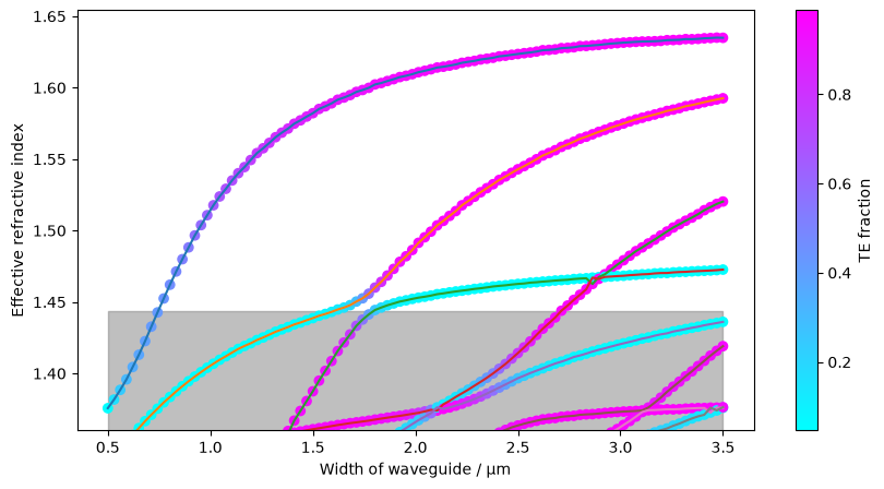
The graph shows a TE mode emerging (getting a greater effective refractive index than the box) at a width of ~750nm. The second mode emerges at a wavelength of ~1700nm. Thus, the waveguide is a single mode waveguide with a width within the range from ~750nm to 1700nm.

The second mode is at the width at which it emerges a TM-mode, but shows for slightly wider waveguides an anti-crossing with the emerging TE-mode. After this anti-crossing, the mode with the second highest effective refracteive index is TE10-mode, while the TM00-mode keeps existing in the system with an effective refractive inded slightly above the cutoff. At a width of ~2600nm, a third TE-mode starts being guided.